Databricks is rolling out the second version of its MLflow platform that will accelerate the production and deployment of Machine Learning models at scale by introducing advanced features. MLflow 2.0 simplifies developing and managing Machine Learning operations by reducing the manual work related to iteration and deployment of models, providing production-grade MLflow pipelines, and presenting the users with well-defined pipeline templates.

The platform supports both Notebook and IDE for analyzing data, writing code, and productionization. One can use the Notebook to trigger the pipeline execution smoothly. Moreover, MLflow enables you to ingest and validate data before you proceed with ETL, and helps you validate, monitor, and deploy your model — all on one platform.

The followings are the main components of MLflow:

It provides API and UI for recording code, data sets, parameters, etc. By using this feature, you can track specific pipelines being used for different Machine Learning models.

MLflow Projects uses a standard format for packaging data science code that enables the users to run that code on any platform. Besides making the code reusable, it also manages the library issue and configuration of files for data scientists.

MLflow takes care of model packaging, formatting, and relevant tools. By doing this, it enables the model to serve in diverse environments like Azure, AWS, etc. This component contains high volumes of metadata and model signatures.

The Registry provides the API and UI required for the central management of the ML model and its lifecycle. It presents details like model annotation, lineage, version, and stage transitions.

MLflow pipelines is a new addition to the MLflow platform; it provides production-grade pipeline templates to users to standardize the model development process and make it faster and easier. It also contains step-by-step instructions regarding building data pipelines for Machine Learning models.

Let’s try to understand how MLflow works with the help of a demo. The data set, being used for the demo, is related to drawing New York City taxi fare predictions. We are aiming to predict the fare amount for the potential passengers. For this purpose, we will use variables like pick-up and drop-off dates and times, trip distances, zip codes, hours, and the duration of the trips in minutes, etc. Moreover, we are using Databricks platform to assist with the process.

For preprocessing, we will determine some standard procedures beforehand. For instance, to calculate the trip duration, we use drop-off and pick-up values. The trip duration is used to make sense if the pickup and drop off times don’t add up. Numerous factors can be responsible for this like getting stuck in the traffic while the meter keeps running or making the taxi wait outside before you finally ride it.

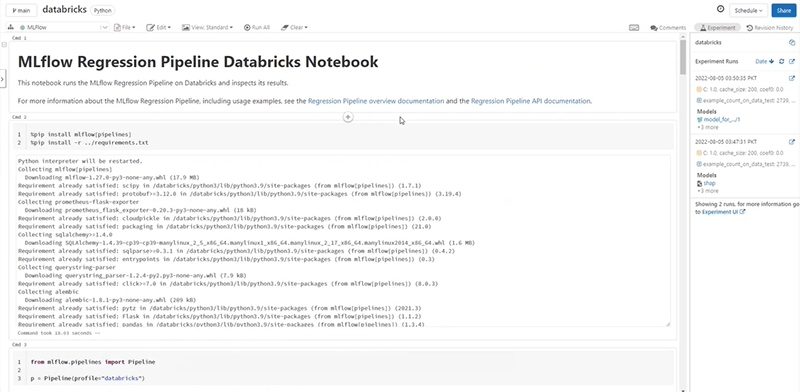
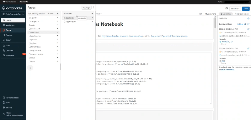
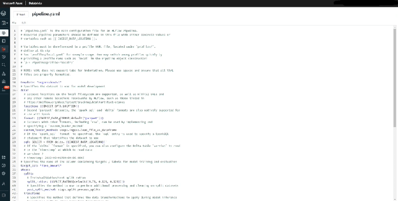
We begin by cloning a template. The most essential file in this regard is the pipeline.yaml. In this file, each and every step has been configured. It provides all the data specifications and related to data processing and evaluation.

The following book is defined by MLflow. In the first column, we are installing all the basic libraries needed to run the code.

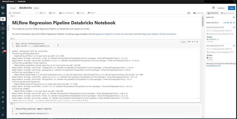
In the next step, we are developing the Databricks pipeline.

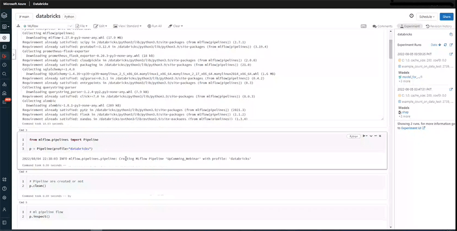
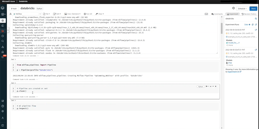
We are using the p.clean function to ensure that the pipeline has been created successfully and there is nothing cached.

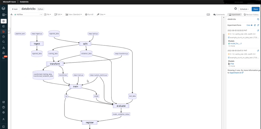
P.inspect shows the whole transformation and all the processes we undertake in a mapped form i.e., the overall flow of our task.

Now, we will describe the path for data ingestion, defined in the databricks.yaml file, with details like the source of the data, its format, the split ratio, etc.

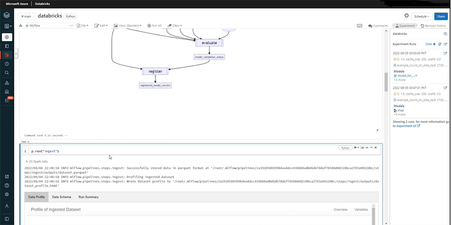
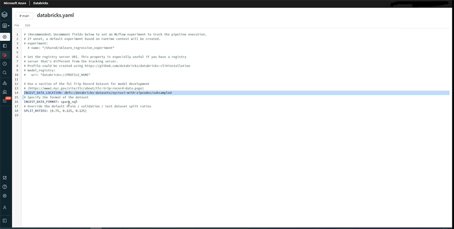
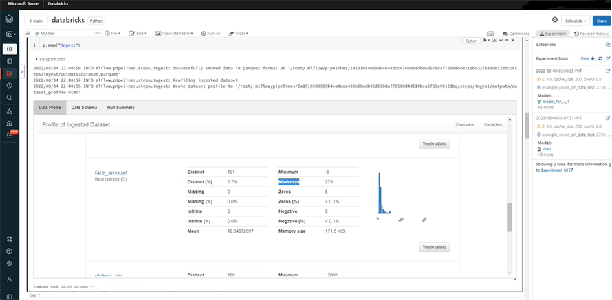
Once we run it, it will provide the schema with data type for each column.

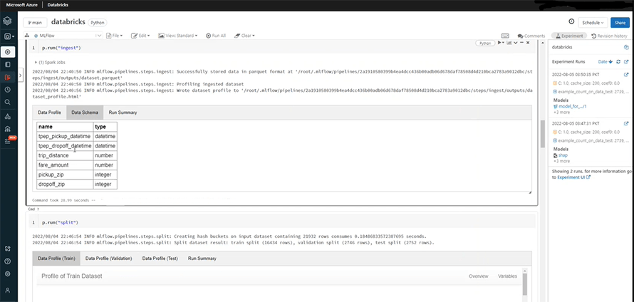
In data profile, you can get the overview on the number of variables, observations, and cells.

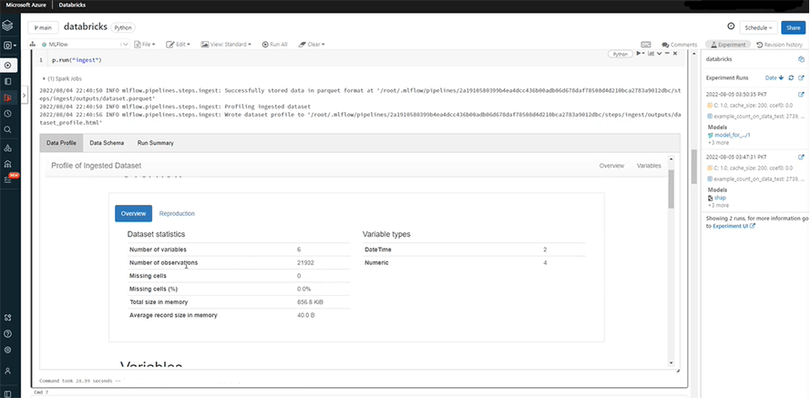
Data profile also defines each variable precisely.

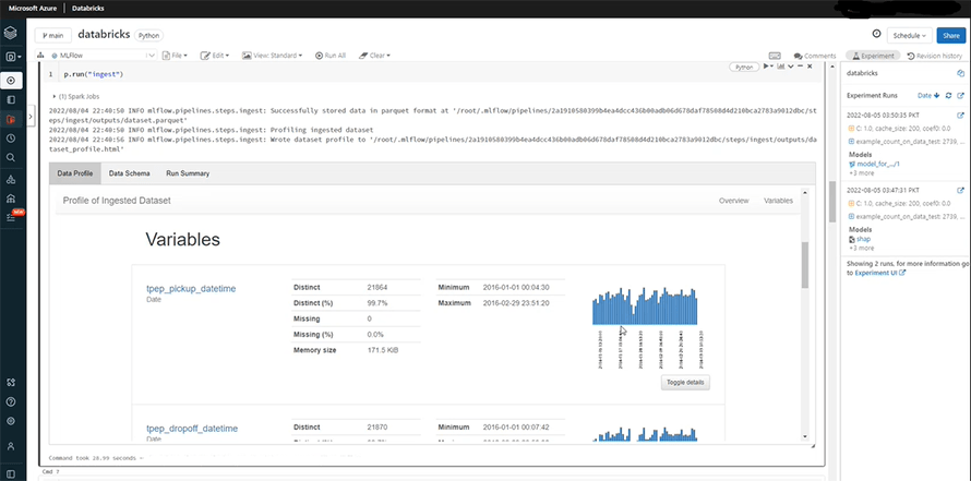
It also shows the mean, negative, maximum, and the minimum value.

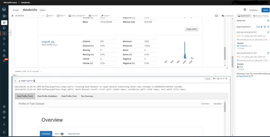
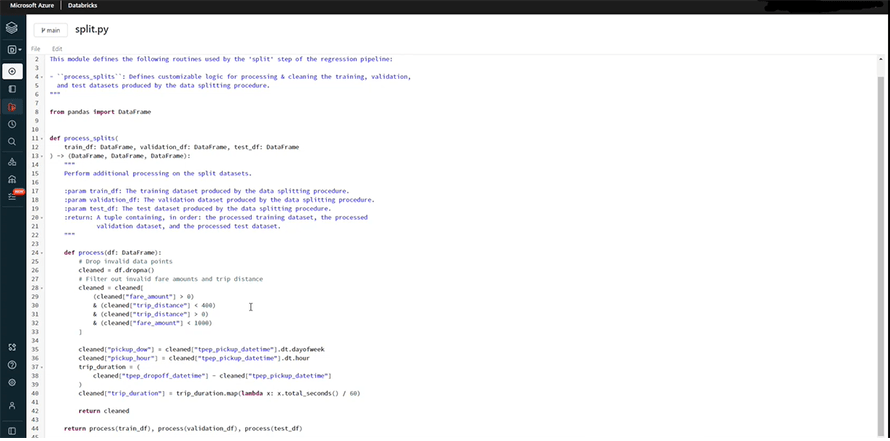
We are doing some preprocessing for the split function in the following image.

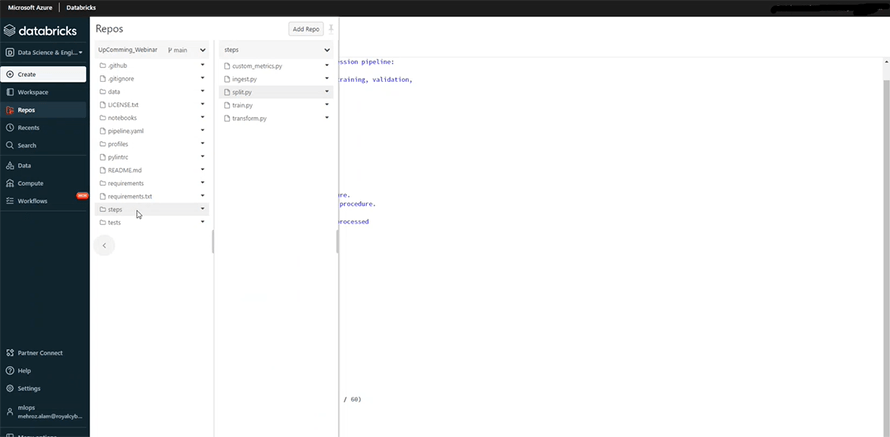
In the Repos, we open the steps and access the split.py class. Its purpose is to remove anomalies and clean the data.

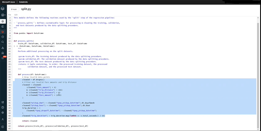
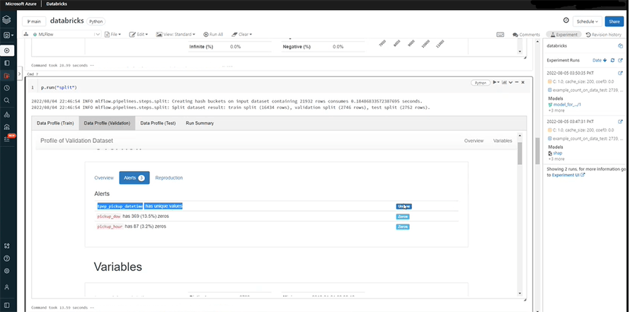
The split function divides the data into three parts: train (for training the model), validate (for tuning hyperparameters), and test (for checking performance of the model). You can see the preprocessing in the highlighted area below:

The split section also provides some alerts like columns with unique values, and the number of zero values in different columns.

The solution automatically removes all the records with fare values that are negative or less than zero.

The data segregated and cleaned by split function will now go through the transformation phase. Transformation shows up in the transform file – in three columns. It increases the accuracy of the data and prepare it for model training.

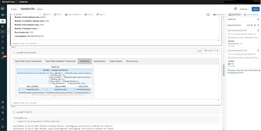
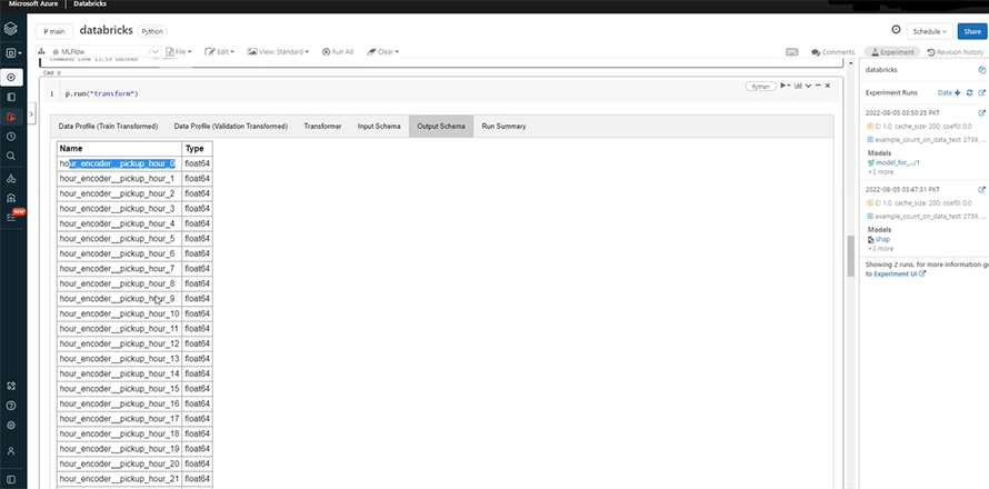
You can see the multiple features provided below, including input and output schema, and run summary.

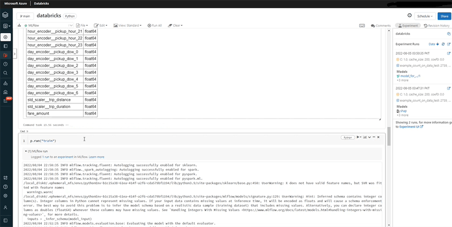
We can now train the model by running the following part.

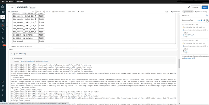
Once the models are trained, you’ll be able to see the error rates if you run the “evaluate”command.

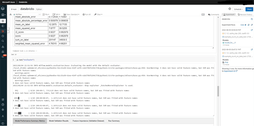
We can now compare both models to find the reason behind the difference in the error rates.

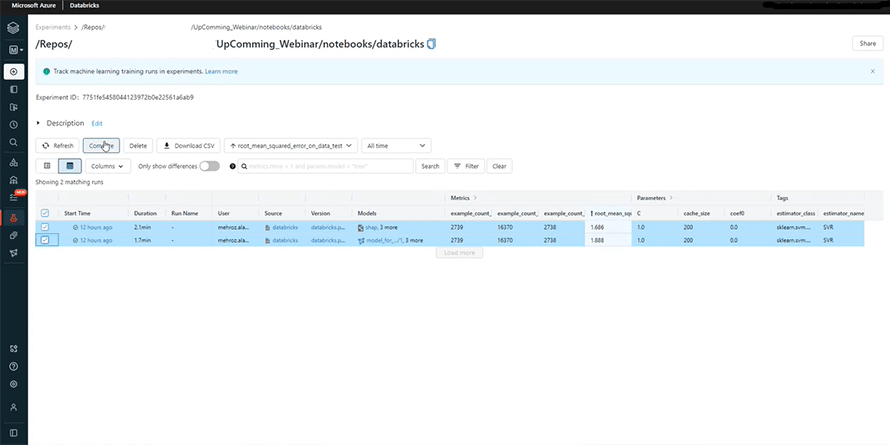
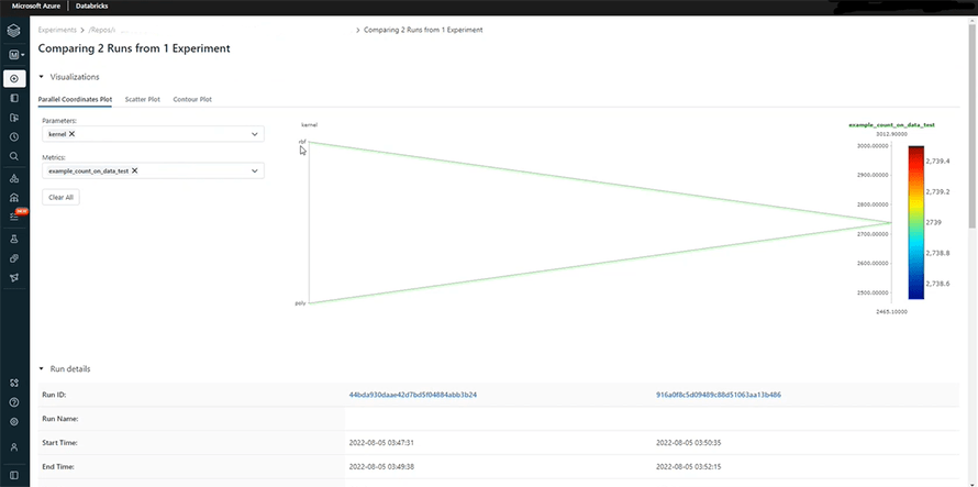
As you may see, we have used rbf and poly for the first and second models, respectively. This is precisely the cause behind the showing up of different error rates. The rbf model seems to be performing better as its error rate is decreasing gradually on the graph. You can also draw the comparison between your parameters and the error function on the scatter plot section, right next to the parallel coordinate plot. It is a very smart and efficient alternative to writing multiple commands repeatedly on your notebook to fetch the same comparison.

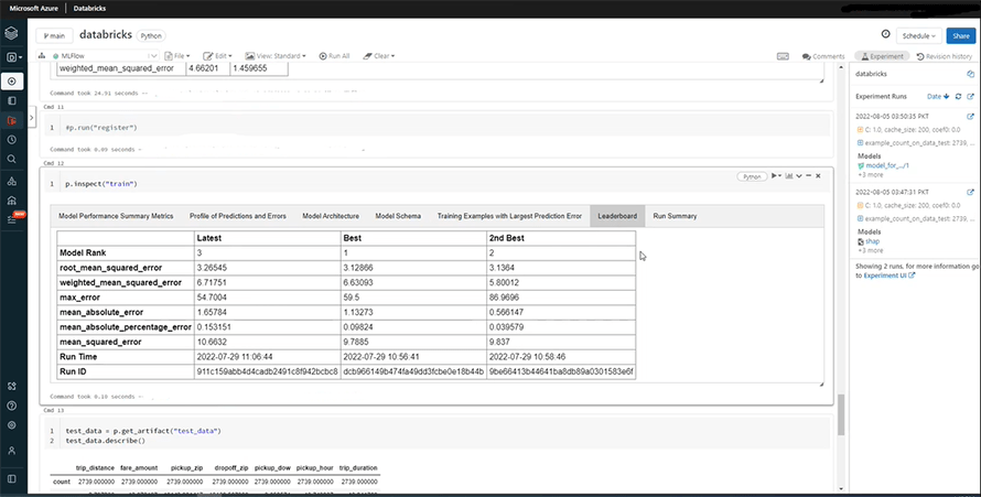
The leaderboard (shown below) is a very useful tool for assessing different Machine Learning models and identifying which one of them is performing best. It ranks the models on the basis of their performance along with their run ids. In this way, it provides users with a strong contingency plan which can be taken up if the model of choice fails to function.

Once you train the model, you can check the artifacts. This section contains the relevant codes, data pipelines, and ingested data of all the runs or features.

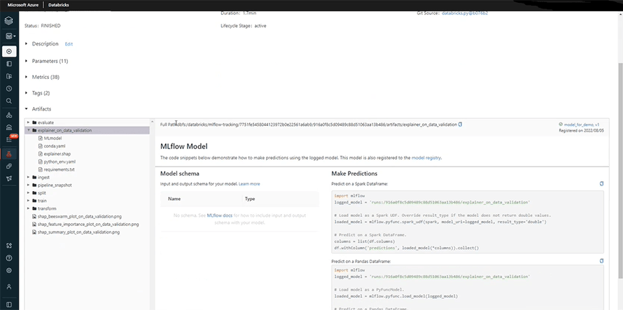
For instance;

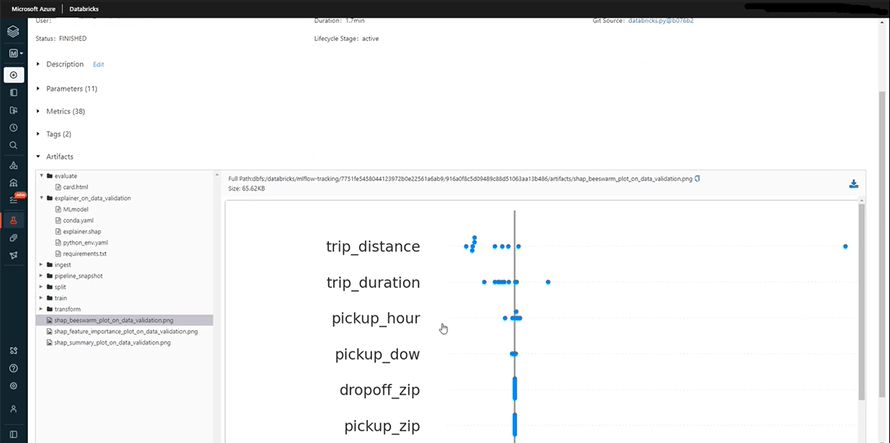
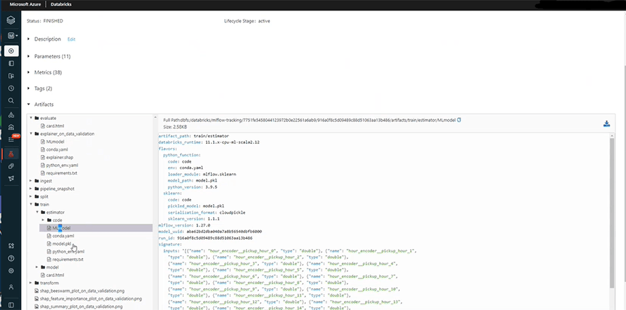
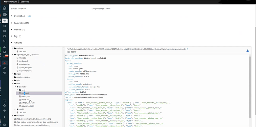
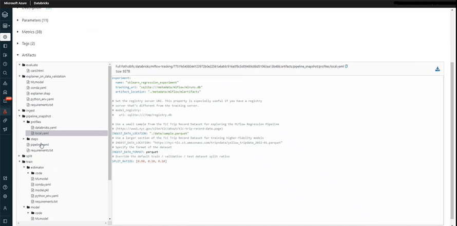
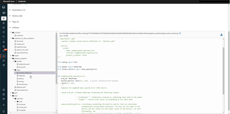
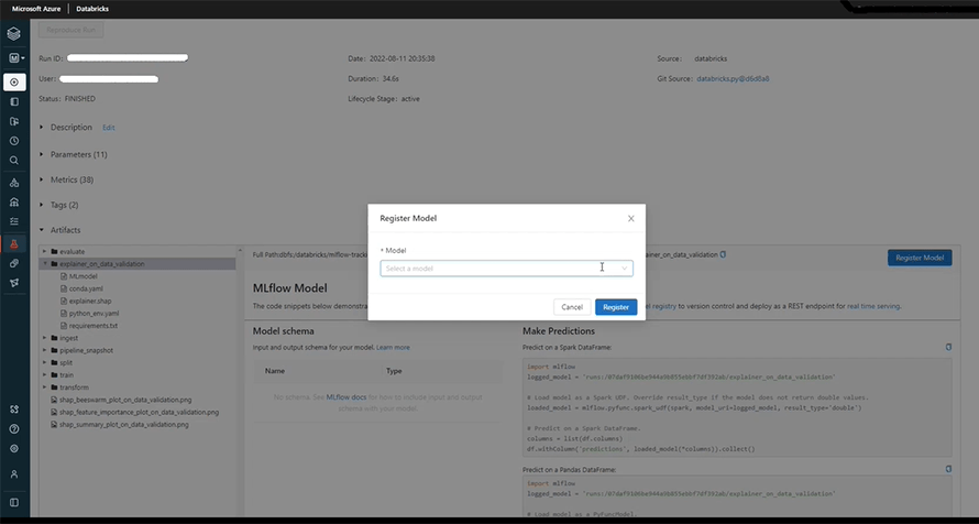
Finally, we can test our model to check its accuracy in the following section and observe predictions. For this, we need to click the ‘Register Now’ option at our right side.

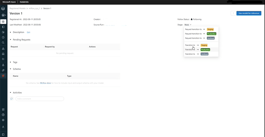
Once our model is registered, we can click on the ‘None’ option to turn proceed to the staging stage. Staging will help us in testing the model after which we can deploy it to production.

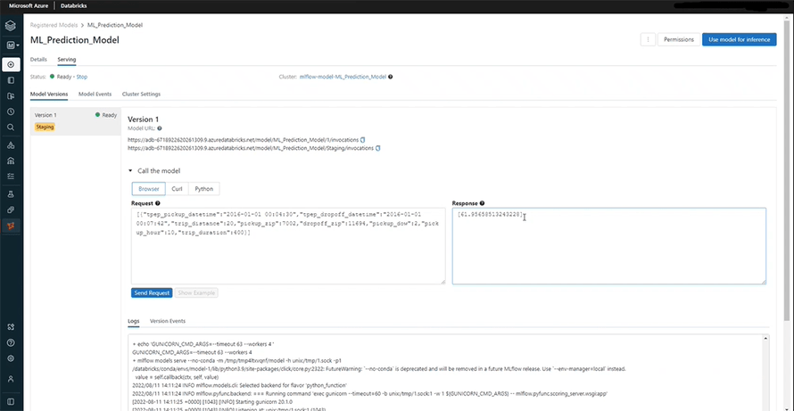
Here, you can see the final results.

By introducing MLflow 2.0, Databricks is taking things to the next level as deploying efficient Machine Learning models is not so difficult anymore.

Royal Cyber provides intelligent Machine Learning-based AI solutions to global businesses. Its data science and analytics teams have comprehensive knowledge and experience in working with data technologies introduced by Databricks and Apache Foundation. If you are still confused about the usage of the MLflow platform, you can contact our data scientists and discuss your queries.